Key Moments
Stanford AA274A Principles of Robotic Autonomy | Autumn 2019 | Trajectory Optimization
 Stanford Online
Key Moments
Trajectory optimization enables robots to find efficient paths, but many methods struggle with real-time computation and complex constraints. Differential flatness offers a computationally efficient solution for a broad class of systems.
Key Insights
The core problem of trajectory optimization is finding a time-history of states and controls that connects an initial to a final state while satisfying system constraints and optimizing a cost function.
Euler's method provides a simple, albeit not the most accurate, way to numerically solve differential equations by discretizing time and approximating derivatives.
The cost function in optimal control typically has two parts: a running cost (integral of control effort or time) and a final cost, allowing designers to prioritize objectives like time or energy.
Open-loop control is a pre-calculated trajectory that depends only on time, while closed-loop control continuously adjusts based on the current state, offering robustness against model errors.
Differential flatness is a property of certain systems that allows for the computation of feasible trajectories and control inputs by considering a subset of state variables (flat outputs) and their derivatives, avoiding direct solution of differential equations.
For differentially flat systems, trajectory optimization can be simplified into a three-step process: converting initial/final conditions to the flat output space, creating a smooth curve in the flat output space (e.g., using polynomial interpolation), and then mapping back to state and control inputs.
Understanding the trajectory optimization problem
The fundamental challenge in robotic autonomy addressed here is trajectory optimization: given an initial state (position, orientation) and a desired final state, how does one find a time-series of states and control inputs that connects these two points while adhering to system dynamics and constraints? These constraints can be kinematic (like non-slipping conditions for wheeled robots) or related to control input limits. Beyond mere feasibility, the goal is often to optimize a cost function, such as minimizing travel time, control effort, or a combination thereof. This problem is central to robotic autonomy and requires understanding the underlying dynamic models and how to manipulate them.
Numerical solution of differential equations: Euler's method
Robotic motion is described by differential equations. To make these computationally tractable, numerical methods are employed. Euler's method is a simple approach to discretize time, approximating a derivative (e.g., ẋ(t)) as (x(t + Δt) - x(t)) / Δt. This allows the differential equation to be rewritten as x(t + Δt) = x(t) + Δt * ẋ(t). By iteratively applying this formula starting from an initial condition, one can estimate the system's state over time. While straightforward, this method involves a trade-off: smaller time steps (Δt) increase accuracy but also computational cost, while larger steps reduce computation but introduce significant errors. This numerical approach is essential for simulating and controlling robotic systems where analytical solutions are often impossible.
Formulating the optimal control problem
An optimal control problem involves finding a control input history U(t) and corresponding state trajectory X(t) that minimize a cost function J. This cost function typically consists of two components: a running cost, often an integral over time (e.g., ∫ G(X(t), U(t)) dt), representing cumulative costs like energy consumption or time elapsed, and a final cost, H(X(T_f)), which penalizes the system's state at the terminal time T_f. The running cost's additive structure, often expressed as an integral, is crucial for efficient computation, particularly in dynamic programming. The final cost, for example, could penalize the deviation from a desired final state. The choice and weighting of these cost functions are determined by the designer based on the specific performance objectives for the robot, balancing factors like speed, energy efficiency, and accuracy.
Open-loop vs. closed-loop control
Two main approaches to control are open-loop and closed-loop. Open-loop control generates a pre-calculated trajectory and control signal that depend only on time, assuming the system will perfectly follow this plan. This is computationally efficient but brittle; any deviation from the nominal model due to disturbances or model inaccuracies will lead to errors that are not corrected. Closed-loop control, conversely, continuously measures the system's state and adjusts the control input accordingly. This feedback mechanism makes it robust to model uncertainties and external disturbances, allowing the robot to correct its path and return to the desired trajectory. While closed-loop control is more robust, it is generally more computationally demanding as it requires online state estimation and control computation.
Differential flatness: Simplifying trajectory computation
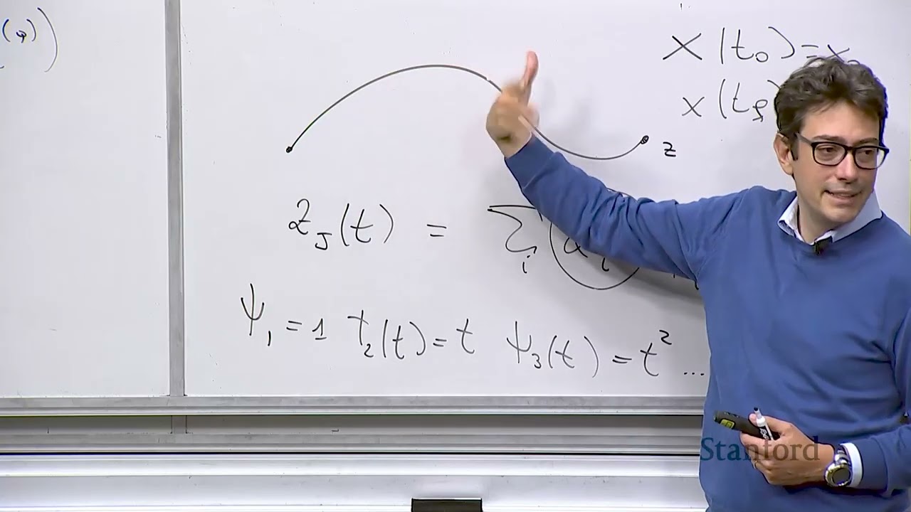
Differential flatness is a property of a class of nonlinear systems that significantly simplifies trajectory optimization. A system is differentially flat if there exists a set of outputs (called flat outputs) and their derivatives such that all system states and control inputs can be expressed as functions of these flat outputs and their derivatives, without needing to integrate the system's differential equations. For instance, in a simple car model, the (x, y) position of the rear axle can be considered flat outputs. From these, the car's orientation (θ) and control inputs (velocity V, steering angle φ) can be uniquely determined. This property is powerful because it transforms a complex dynamic problem into a simpler geometric one: planning a path in the lower-dimensional flat output space and then using algebraic mappings to recover the full state and control trajectories. This dramatically reduces computational complexity, making real-time trajectory recalculation feasible.
Applying differential flatness for practical trajectory planning
The practical application of differential flatness involves a straightforward three-step algorithm. First, initial and final conditions of the system's states and inputs are transformed into equivalent conditions for the flat outputs and their derivatives. Second, a smooth curve is generated in the flat output space, typically using polynomial interpolation (e.g., cubic splines) to connect the transformed initial and final conditions. This planning step is computationally inexpensive as it operates in a lower-dimensional space and doesn't require solving differential equations. Finally, an inverse mapping (provided by the system's structure) is used to translate the planned flat output trajectory back into the actual state and control input trajectories for the robot. This approach is computationally efficient, often allowing for high-frequency trajectory updates necessary for autonomous systems operating in dynamic environments.
Challenges and extensions of differential flatness
While powerful, differential flatness has limitations. There is no general algorithmic method to determine if an arbitrary system is differentially flat, making its application non-trivial. Furthermore, incorporating complex constraints, such as input limits (e.g., maximum velocity), requires transforming these constraints into the flat output space, which can be challenging. Techniques like time-scaling can be used to satisfy input constraints by adjusting the pace along the planned trajectory. For optimizing trajectories, beyond mere feasibility, one might minimize higher-order derivatives like jerk (the third derivative of position) to ensure smoother, more controllable paths. This often involves formulating an optimization problem in the flat output space with an appropriate cost function.
Mentioned in This Episode
●Software & Apps
●Organizations
●Books
●Concepts
●People Referenced
Common Questions
Trajectory optimization is the problem of finding a path (a time history of states, including position and orientation) that connects an initial state to a desired final state while satisfying system constraints, such as kinematic or control limits. It often involves optimizing a cost criterion, like minimizing time or control effort.
Topics
Mentioned in this video
A method used for trajectory optimization, particularly applicable to a wide class of systems like quadrotors and aerial vehicles. It allows for efficient path calculation by decoupling the problem into finding a path for a subset of state variables and then deriving the control inputs.
A method for solving complex problems by breaking them down into simpler subproblems, developed by Richard Bellman.
A method developed from the Soviet school of optimal control theory, used for solving optimal control problems.
A basic kinematic model of a car used as an example to illustrate differential flatness. It has two rear wheels and steerable front wheels.
An American mathematician known for his work on dynamic programming, which emerged from the American school of optimal control.
A researcher from Caltech whose work is referenced for practical applications and theoretical overviews of differential flatness.
Authors of the primary reference book for the course, 'Robotics: Modelling, Planning and Control'.
A theoretical reference book for differential flatness, noted for its mathematical rigor.
A less mathematical version of a reference book on differential flatness compared to Levine's book.
The main textbook for the course, specifically Chapter 11 covers trajectory optimization.
More from Stanford Online
View all 148 summaries 104 min
Stanford CME295 Transformers & LLMs | Autumn 2026 | Lecture 2 - Large Language Models
 76 min
Stanford AA274A Principles of Robotic Autonomy | Autumn 2019 | Overview, Mobile Robot Kinematics
 78 min
Stanford AA274A Principles of Robotic Autonomy | Autumn 2019 | Advanced Trajectory Optimization
 79 min
Stanford AA274A Principles of Robotic Autonomy | Autumn 2019 | Trajectory Tracking
Ask anything from this episode.
Save it, chat with it, and connect it to Claude or ChatGPT. Get cited answers from the actual content — and build your own knowledge base of every podcast and video you care about.
Get Started Free