Key Moments
Stanford AA203 Optimal and Learning-Based Control | Spring 2026 | Lecture 12: Feasibility of MPC
 Stanford Online
Want to know something specific about what's covered?
We've already dissected every moment. Ask and we will deliver (with timestamps).
Key Moments
MPC guarantees persistent feasibility and stability by carefully selecting terminal sets and costs, but naive trajectory tracking formulations can lead to oscillations. Explicit MPC offers offline computation, potentially simplifying validation.
Key Insights
If the terminal set (X_f) is a control invariant set for the system, then Model Predictive Control (MPC) is guaranteed to be persistently feasible.
The origin (state zero) is always a control invariant set, ensuring persistent feasibility if chosen as the terminal constraint, but can lead to suboptimal control effort.
A key theorem for MPC stability states that if the terminal set (X_f) is control invariant and a specific Lyapunov-like condition involving the terminal cost (P) is met, the closed-loop system is asymptotically stable with domain of attraction X0.
For an asymptotically stable system, choosing X_f as the maximally positive invariant set and P as the solution to the Lyapunov equation ensures stability.
For an unstable system, choosing X_f as the positive invariant set for the closed-loop LQR dynamics and P as the solution to the Riccati equation ensures stability.
Naive MPC formulations for trajectory tracking penalizing state deviation and control effort can lead to oscillations; a better approach involves penalizing deviations in control *changes* (delta u).
Ensuring persistent feasibility through control invariant sets
The lecture begins by revisiting the concept of persistent feasibility in Model Predictive Control (MPC), emphasizing the need for the control loop to have at least one feasible solution at each time step. A crucial lemma establishes that if the one-step controllable set to X1 (a feasible set from stage one) is control invariant, then MPC is persistently feasible. While this lemma itself isn't directly tunable, it serves as a stepping stone to a more practical theorem: if the terminal set (X_f), a parameter actively tuned in MPC, is a control invariant set for the system, then MPC is guaranteed to be persistently feasible. This is because a control invariant set ensures that from any state within the set, there exists a feasible control to transition back into the set. The origin (state zero) is always a trivial control invariant set, guaranteeing feasibility if chosen as X_f. However, using the origin as the sole terminal constraint can be overly restrictive and lead to excessive control effort, prompting the need for more sophisticated choices of X_f.
The role of the terminal set in guaranteeing feasibility
The proof connecting the terminal set X_f to persistent feasibility involves showing that if X_f is control invariant, then recursively, X_{n-1}, X_{n-2}, ..., and finally X1 also become control invariant. This recursive property, when applied to the previously stated lemma about X1, confirms that if X_f is control invariant, the MPC loop will always find a feasible solution. The choice of X_f is a critical design knob for ensuring persistent feasibility. While the origin is the simplest control invariant set, it is often suboptimal. The lecture hints at more advanced methods for computing larger, more relaxed control invariant sets, which will be explored later and in problem sets. This theoretical guarantee of feasibility is fundamental to reliable MPC operation.
Establishing stability using Lyapunov functions
Transitioning from feasibility to stability, the lecture introduces Lyapunov stability theory as a tool to prove that MPC can drive the system to an equilibrium point (typically the origin). A Lyapunov function, V(x), is an 'energy-like' function that is zero at the equilibrium, positive elsewhere, and strictly decreases along system trajectories. If such a function can be found, it implies that the system's state will converge to the minimum of V, which is the equilibrium point. The lecture highlights that this method allows proving stability without explicitly solving the system's differential or difference equations, which can be complex. The core idea is to demonstrate energy dissipation, leading the system towards a stable state. The challenge often lies in finding a suitable Lyapunov function.
Lyapunov stability theorem for MPC
A central theorem for MPC stability is presented, assuming a quadratic cost function, positive definite control and state penalties (Q, R), and a positive definite terminal cost (P). Crucially, it requires the terminal set X_f to be control invariant and satisfies a specific Lyapunov-like condition: for all x in X_f, there exists a control u such that the change in the terminal cost P from the current state to the next state (after applying control u) is negative, i.e., P(ax+bu) - P(x) <= -c(x,u), where c(x,u) is a positive term related to the stage cost. If these conditions hold, the origin is asymptotically stable with a domain of attraction X0. The proof demonstrates that the optimal MPC cost-to-go function, J*(x), can serve as a Lyapunov function, satisfying the necessary properties, thereby guaranteeing stability.
Actionable tuning for stability and feasibility
The lecture provides practical guidance on selecting tuning parameters (terminal set X_f and terminal cost P) based on the stability theorem. If the system's dynamics matrix 'a' is asymptotically stable, X_f can be chosen as the maximally positive invariant set for the uncontrolled system (x_{t+1} = ax_t), and P can be the solution to the Lyapunov equation. This setup leverages the system's natural stability. If 'a' is unstable, X_f is chosen as the positive invariant set for the closed-loop LQR dynamics (with gain F_infinity), and P is the solution to the Riccati equation. These choices provide a procedural way to tune MPC for both persistent feasibility and asymptotic stability, ensuring that the system converges to the origin.
Explicit MPC: offline computation for real-time performance
Beyond online optimization, the concept of explicit MPC is introduced. In this approach, the MPC control law is pre-computed offline and represented as a piecewise affine function over a polyhedral partition of the state space. This means that at runtime, instead of solving an optimization problem, the system performs a state space lookup to find the appropriate affine control law. This method offers significant advantages in terms of avoiding online optimization challenges, simplifying validation for safety-critical applications, and potentially reducing computational delays. However, the complexity of the state-space partition can sometimes lead to very large lookup tables. Modern online optimizers have become so efficient that, in many cases, solving the optimization problem online is faster than performing a lookup in a massive table, making explicit MPC less universally adopted than it once was.
Addressing trajectory tracking with MPC
Finally, the lecture touches upon using MPC for trajectory tracking, a common application where the goal is to follow a reference trajectory rather than converge to a fixed point. A naive approach, penalizing deviations from the reference state and control effort, is shown to be problematic. If the system perfectly tracks the reference (zero state error), the cost becomes dominated by control effort, potentially leading to oscillations as the MPC tries to minimize control input, which in turn increases tracking error. A more effective formulation reframes the problem by penalizing deviations in the *change* of control inputs (delta u) rather than the absolute control inputs. This allows for maintaining a constant, non-zero control effort (like engine thrust) required for perfect tracking, while penalizing unnecessary fluctuations in control.
Mentioned in This Episode
●Software & Apps
Common Questions
Persistent feasibility in MPC ensures that a feasible solution exists at every step of the control loop. This means that at each decision point, the system can find a valid control action that respects all constraints and dynamics.
Topics
Mentioned in this video
A numerical computing environment and programming language used for algorithm development, data visualization, and analysis, mentioned as a tool for solving control problems.
A toolbox likely related to Model Predictive Control (MPC) and related control theory concepts, used for computing control sets and other related tasks.
More from Stanford Online
View all 135 summaries 74 min
Stanford AA203 Optimal and Learning-Based Control | Spring 2026 | Lecture 16: Fundamentals of RL
 80 min
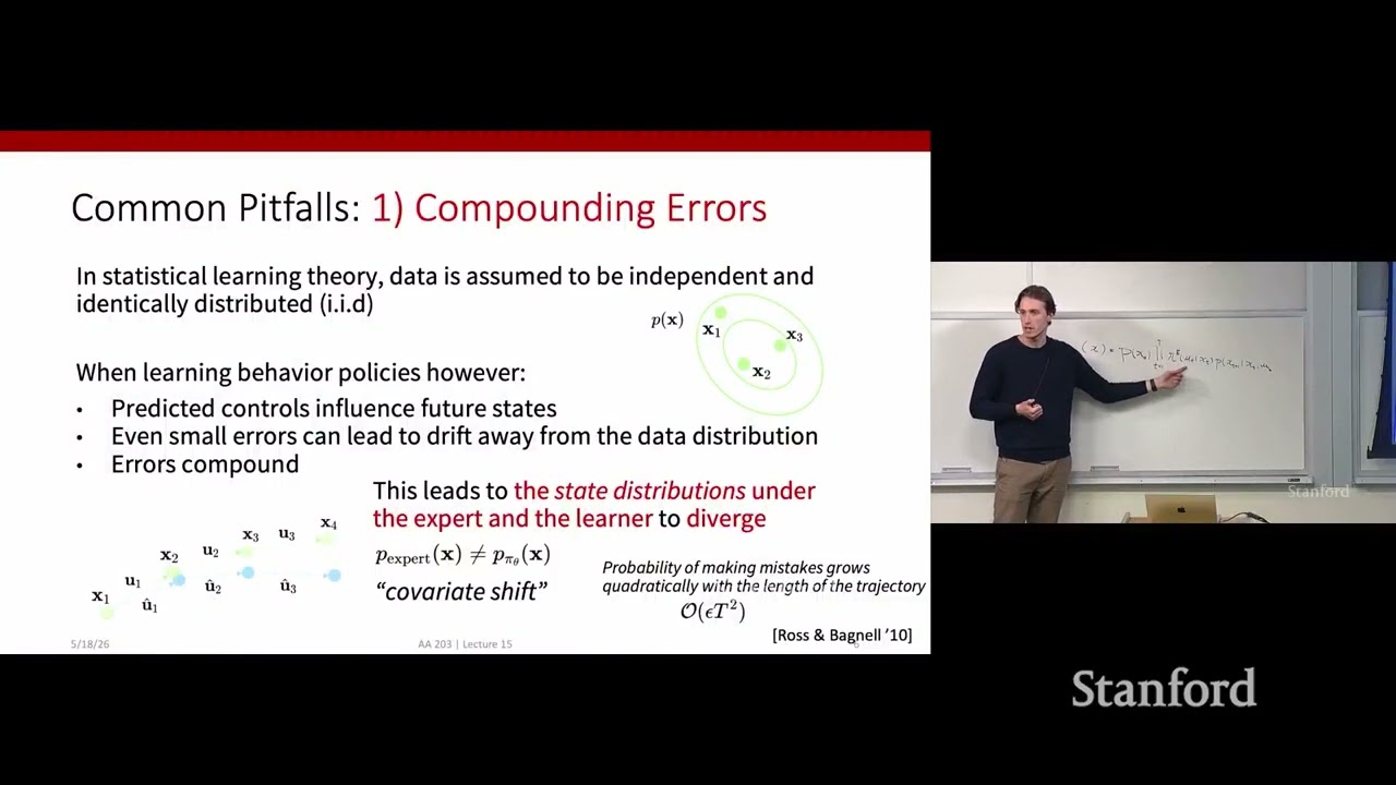
Stanford AA203 Optimal and Learning-Based Control | Spring 2026 | Lecture 15: Imitation Learning
 78 min
Stanford AA203 Optimal and Learning-Based Control | Spring 2026 | Lecture 17: RL Value-Based Methods
 81 min
Stanford AA203 Optimal and Learning-Based Control | Spring 2026 | Lecture 18: RL Policy Optimization
Ask anything from this episode.
Save it, chat with it, and connect it to Claude or ChatGPT. Get cited answers from the actual content — and build your own knowledge base of every podcast and video you care about.
Get Started Free