Key Moments
Stanford AA203 Optimal and Learning-Based Control | Spring 2026 | Lecture 7: Dynamic Programming
 Stanford Online
Want to know something specific about what's covered?
We've already dissected every moment. Ask and we will deliver (with timestamps).
Key Moments
Dynamic programming allows for optimal closed-loop control policies, but its computational demands scale exponentially with state dimension, making it impractical for complex systems without approximation.
Key Insights
Direct methods for optimal control are more popular in robotics due to advances in algorithms and hardware, enabling on-the-edge computation.
The principle of optimality states that an optimal policy's tail is also optimal for the truncated problem, enabling efficient computation by reusing solutions to subproblems.
Dynamic programming solves for optimal closed-loop policies by working backward in time, starting from a known terminal cost.
The curse of dimensionality means dynamic programming's computational cost scales exponentially with the state space dimension (e.g., 10^D), rendering it intractable for high-dimensional problems without approximations.
The Linear Quadratic Regulator (LQR) problem, a specific case solvable by dynamic programming, results in a linear feedback control law and quadratic cost-to-go, simplified by recursive Riccati equations.
While dynamic programming provides globally optimal closed-loop solutions, its application requires careful problem formulation (modeling) and often necessitates approximate methods for scalability.
Open-loop vs. closed-loop control policies
The lecture begins by contrasting open-loop and closed-loop optimal control methods. Open-loop methods compute a sequence of control inputs over time, assuming the system follows a nominal trajectory. Indirect methods derive necessary conditions for optimality, often leading to a two-point boundary value problem, while direct methods discretize the problem and solve it as a nonlinear optimization problem. Direct methods are currently more popular in robotics due to computational advances. Closed-loop methods, however, aim to find an optimal control policy that maps any given state at any time to the optimal control input. This makes them more robust to disturbances and model mismatches, as the policy dictates the correct action even when the system deviates from the nominal trajectory. The trade-off is that closed-loop methods, like dynamic programming, are computationally more intensive.
The principle of optimality
The core concept enabling dynamic programming is the principle of optimality. This principle, derived from the additive nature of the cost function, states that if a sequence of decisions is optimal for a multi-step problem, then the portion of that sequence from any intermediate step onwards must also be optimal for the subproblem starting at that intermediate step. This is proven by contradiction: if a tail path were not optimal for its subproblem, a better tail path would exist, which could then be substituted to create a better overall path, contradicting the initial assumption of optimality. This principle allows for reusing solutions to subproblems, significantly reducing computational effort compared to re-solving from scratch at each step. The key is that the optimal policy for the future depends only on the current state, not on how that state was reached.
Dynamic programming algorithm and backward recursion
Dynamic programming provides a procedural algorithm to solve for optimal closed-loop policies. It operates by working backward in time, starting from the terminal cost at the final stage (N). At each preceding stage (k), it determines the optimal control by minimizing the sum of the immediate stage-wise cost and the optimal cost-to-go from the next state (k+1). This 'cost-to-go' is already known from the previous backward step. This backward recursion allows the algorithm to build up the optimal policy from the end to the beginning. While the concept is straightforward, applying it requires discretizing both time and the state space, which can lead to computational challenges. The process involves solving a minimization problem at each state-time pair to find the optimal control and the associated cost-to-go.
The curse of dimensionality and computational challenges
A major challenge with dynamic programming is the 'curse of dimensionality.' The computational cost grows exponentially with the dimension of the state space. If the state is D-dimensional and each dimension is discretized into M levels, the number of states to consider becomes M^D. This means that for even moderately complex systems with higher-dimensional state spaces (e.g., robotics with multiple joints), the number of computations required becomes astronomically large, rendering the exact dynamic programming solution computationally infeasible. This necessitates the use of approximation techniques, which are crucial for applying dynamic programming to real-world problems and form the basis for learning-based control methods.
Application to the Linear Quadratic Regulator (LQR)
The lecture illustrates dynamic programming with the Linear Quadratic Regulator (LQR) problem. This problem involves linear system dynamics and a quadratic cost function (penalizing state deviations and control effort). The objective is to drive the system to the origin with minimal cost. For LQR, dynamic programming simplifies significantly. The backward recursion leads to recursive equations for two matrices: the control gain matrix (F) and the cost-to-go matrix (P). The optimal control is found to be a linear feedback of the state (u = Fx), and the cost-to-go remains a quadratic function of the state. These recursive equations, known as Riccati equations, allow for efficient computation of the optimal policy for LQR problems, highlighting how specific problem structures can dramatically simplify dynamic programming.
Modeling and Scalability
The practical application of dynamic programming hinges on two main challenges: modeling and scalability. Modeling involves mapping diverse problems, such as shortest path problems or even DNA sequencing, into the discrete-time, additive-cost formalism required by dynamic programming. This mapping can require considerable ingenuity. Scalability, on the other hand, addresses the computational burden imposed by the curse of dimensionality. Exact dynamic programming is often infeasible for high-dimensional systems. Therefore, approximate dynamic programming techniques are essential. These approximations, often involving methods like function approximation or discretization strategies, aim to reduce the computational load while retaining sufficient accuracy to yield useful control policies. These approximations are a bridge to learning-based control methods discussed later in the course.
Mentioned in This Episode
●Concepts
Dynamic Programming: Key Takeaways
Practical takeaways from this episode
Do This
Avoid This
Common Questions
Open-loop control computes a predetermined sequence of controls based on time, assuming a perfect model. Closed-loop control, on the other hand, generates a policy that maps states to controls, allowing it to adapt to disturbances or model mismatches by reacting to the current state.
Topics
Mentioned in this video
More from Stanford Online
View all 126 summaries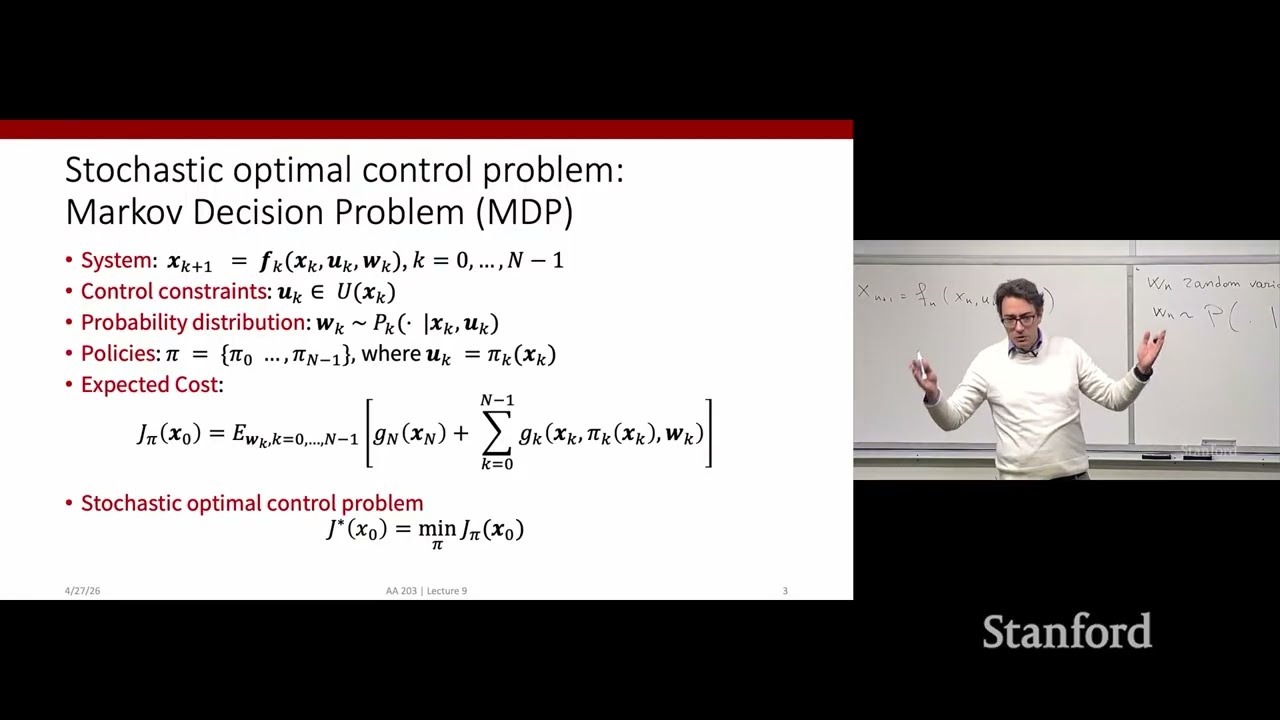 78 min
Stanford AA203 Optimal and Learning-Based Control | Spring 2026 | Lecture 9: Stochastic Dyn. Program
 78 min
Stanford AA203 Optimal and Learning-Based Control | Spring 2026 | Lecture 10: Reachibility Analysis
 81 min
Stanford AA203 Optimal and Learning-Based Control | Spring 2026 | Lecture 6: Optimal Control
 75 min
AStanford AA203 Optimal and Learning-Based Control | Spring 2026 | Lecture 8: Nonlinearity
Ask anything from this episode.
Save it, chat with it, and connect it to Claude or ChatGPT. Get cited answers from the actual content — and build your own knowledge base of every podcast and video you care about.
Get Started Free